Converting an analog image to digital requires 2 independent choices: sampling and quantization. Both determine the memory required for image storage.
Sampling
Sampling fixes the spatial resolution. Resolution is the number of samples per unit length, set by the size of the image sensor element.
Coarse sampling has 3 visible effects: loss of information, pixelation, and aliasing.
Loss of Information
Each cell keeps only one value for the region it covers, so any variation finer than a cell is averaged away and cannot be recovered. Worse with large cells and scenes carrying fine detail.
Pixelation
Each grid cell becomes one flat square of intensity, so a smooth or diagonal edge is replaced by a staircase of these squares. Most visible on high-contrast boundaries such as text against a plain background. Also called the checkerboard effect or blocking.
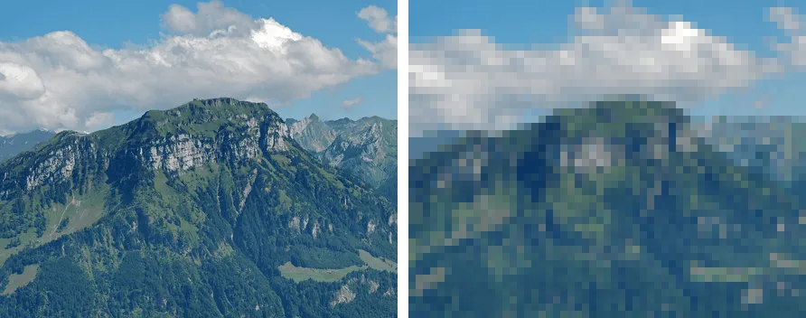
Left: Original. Right: Sampled on a grid 8 times coarser, then shown at the original size. Blocky cells replace fine detail.
Generated from a photo by Hannes Röst, CC BY-SA 3.0.

Aliasing
Aliasing happens when a pattern in the scene repeats faster than the sampling grid can follow. The samples then fit a different, lower-frequency pattern that was never in the scene. That false pattern is the alias.
- The sampling rate is the number of samples per unit distance, one per grid cell.
- Capturing a repeating pattern needs at least 2 samples per cycle of that pattern. This is the Nyquist criterion.
- A pattern with more than 1 cycle per 2 cells is undersampled.
- The alias frequency is the true frequency folded about half the sampling rate. A higher scene frequency gives a lower alias frequency.
- On fine repeating textures the alias shows up as broad curved bands, called moire fringes.
Anti-aliasing removes detail finer than the grid can represent, by optical blur or a low-pass filter, before the image is sampled. This costs high-frequency detail, which is less noticeable when sub-sampling.
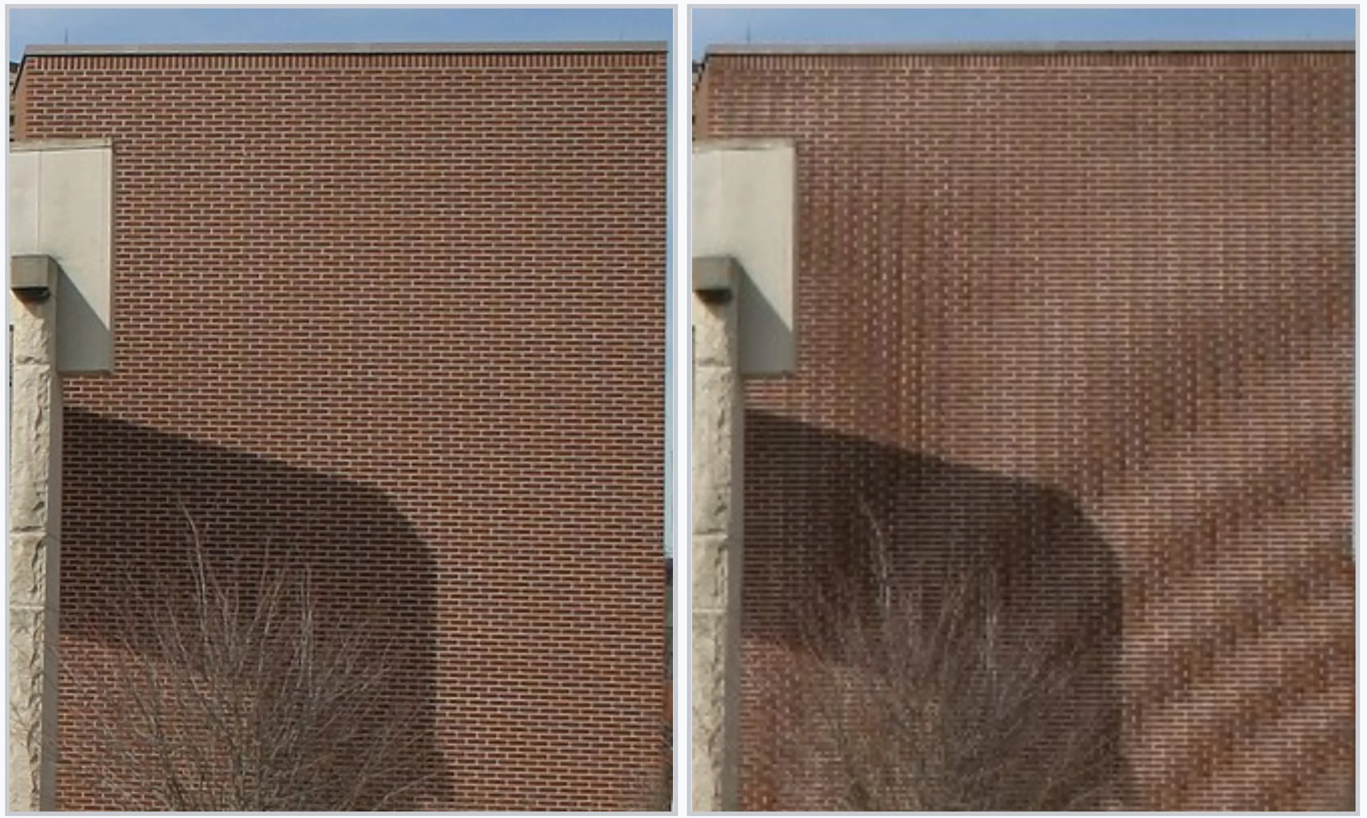
Left: Original image. Right: Aliasing effect. Image by Wikipedia.

Two overlapping railings on a bridge. The beat between the two picket spacings shows up as broad moire bands where the grid is undersampled. Image by Hidalgo944, CC BY-SA 4.0.

Quantization
Quantization fixes the grey-level depth. Grey-level depth is the number of discrete intensity levels, set by the resolution of the analog to digital converter.
Insufficient grey-level depth causes false contouring.
False Contouring
Across a smooth gradient, a band of neighbouring intensities collapses onto one level and renders as a flat region. The jump to the next level shows up as a sharp edge that is not in the scene. These false edges resemble contour lines, most visible in skies and other large smooth areas.
Dithering
Dithering trades spatial resolution for grey-level depth. A device with few output levels approximates an intermediate intensity by mixing the available levels over a small region, which the eye averages at normal viewing distance.
- Each pixel is divided into sub-pixels, each forced to an available level
- The count of sub-pixels at the higher level encodes the target intensity
- A fixed dither matrix sets the order in which sub-pixels switch on, spreading them to avoid visible clumps
Used in newspaper halftoning, laser printing, and exporting photos to a small fixed palette such as GIF.
Worked Example
A bi-level device with output levels and . Target intensity across one block, using the Bayer dither matrix.
Sub-pixel is set to iff .
- has threshold . Since , set to .
- has threshold . Since , set to .
- has threshold . Since , set to .
- has threshold . Since , set to .
2 of the 4 sub-pixels are on, so the block averages , matching the target. The on sub-pixels form a checkerboard.
Error Diffusion
Each pixel is rounded to the nearest available level. The rounding error, the gap between the original value and the chosen level, is spread over neighbouring pixels not yet processed. Those neighbours are nudged toward the value the current pixel could not hold, so the error cancels over a small region instead of building up.
- Pixels are processed in raster order, left to right and top to bottom.
- The error is split by a fixed kernel whose weights sum to , so total intensity is preserved.
- No sub-pixel division, so spatial resolution is preserved.
- The flat bands of false contouring become high-frequency noise, which the eye tolerates better.
Floyd-Steinberg is the common kernel. With the current pixel and the pixels already done, the error is shared as:
Serpentine scanning reverses direction every other row, so the error is not always pushed the same way and directional streaks are avoided.
Worked Example
Bi-level device with levels and . One row of 4 pixels, all at value , using 1D diffusion that passes the whole error to the next pixel.
- Pixel 1’s rounds to , error . Pixel 2 becomes .
- Pixel 2’s rounds to , error . Pixel 3 becomes .
- Pixel 3’s rounds to , error . Pixel 4 becomes .
- Pixel 4’s rounds to .
Output is , mean , matching the target that no single pixel could represent.
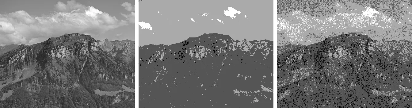
Left: Original greyscale. Centre: Reduced to 4 levels, showing false contouring. Right: Reduced to 4 levels with Floyd-Steinberg error diffusion, trading the flat bands for high-frequency noise. Generated from a photo by Hannes Röst, CC BY-SA 3.0.